bart poisson

=================================================================================================================

The bart poisson command in the BART is used to construct a binary Poisson-disk sampling mask. This type of mask is useful for undersampling k-space data in MRI, which can accelerate the scan.

Purpose: It generates a binary mask that can be applied to k-space data to simulate undersampling.

Poisson-Disk Sampling: is a technique for randomly picking tightly-packed points but with a minimum distance constraint between them.

Where we can view the full usage string and optional arguments with the -h flag.

!bart poisson -h

Usage: poisson [-Y d] [-Z d] [-y f] [-z f] [-C d] [-v] [-e] [-s d] <output> 

Computes Poisson-disc sampling pattern.

-Y size    size dimension 1
-Z size    size dimension 2
-y acc     acceleration dim 1
-z acc     acceleration dim 2
-C size    size of calibration region
-v         variable density
-e         elliptical scanning
-s seed    random seed
-h         help

Examples (python)

# Importing the required libraries
import numpy as np
import matplotlib.pyplot as plt
%matplotlib inline

import cfl
from bart import bart

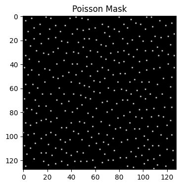
Exmaple 1

-Y 128: Specifies a 128-point size for the first dimension.

-y 10: Specifies an acceleration factor of 10 along this dimension.

poisson_mask_1 = bart(1, 'poisson -Y 128 -y 10').squeeze()

points: 1624, grid size: 128x128 = 16384 (R = 10.088670)

# Visualizing the images using Matplotlib 
plt.figure(figsize=(4,6))
plt.imshow(abs(poisson_mask_1), cmap='gray')
plt.title('Poisson Mask')
plt.show()

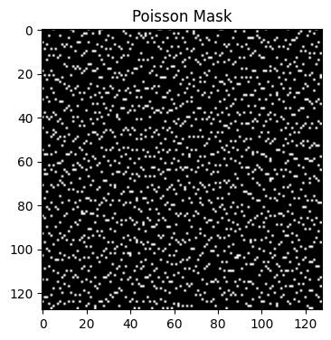
Exmaple 2

-Y 128: Sets the size of dimension 1 (128).

-Z 128: Sets the size of dimension 2 (128).

-y 10: Acceleration factor 10× along dimension 1.

-z 5: Acceleration factor 5× along dimension 2.

poisson_mask_2 = bart(1, 'poisson -Y 128 -Z 128 -y 10 -z 5').squeeze()

points: 327, grid size: 128x128 = 16384 (R = 50.103977)

# Visualizing the images using Matplotlib 
plt.figure(figsize=(4,6))
plt.imshow(abs(poisson_mask_2), cmap='gray')
plt.title('Poisson Mask')
plt.show()

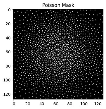
Exmaple 3

-Y 128: Sets the first dimension size to 128.

-Z 128: Sets the second dimension size to 128.

-y 2: Acceleration factor 2× along dimension 1.

-z 2: Acceleration factor 2× along dimension 2.

-v: Enables variable-density Poisson-disc sampling, leading to denser sampling in the center and sparser sampling in outer regions.

poisson_mask_3 = bart(1, 'poisson -Y 128 -Z 128 -y 2 -z 2 -v').squeeze()

points: 1557, grid size: 128x128 = 16384 (R = 10.522800)

# Visualizing the images using Matplotlib 
plt.figure(figsize=(4,6))
plt.imshow(abs(poisson_mask_3), cmap='gray')
plt.title('Poisson Mask')
plt.show()

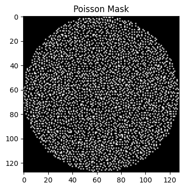
Exmaple 4

-e: Enables elliptical scanning, meaning the sampling follows an elliptical shape rather than a full rectangular grid.

poisson_mask_4 = bart(1, 'poisson -Y 128 -Z 128 -y 2 -z 2 -e').squeeze()

points: 3207, grid size: 128x128x(pi/4) = 12867 (R = 4.012462)

# Visualizing the images using Matplotlib 
plt.figure(figsize=(4,6))
plt.imshow(abs(poisson_mask_4), cmap='gray')
plt.title('Poisson Mask')
plt.show()