bart pattern#
=================================================================================================================
The bart pattern command in the BART calculates the sampling pattern of k-space data by identifying where the data is non-zero. This command is useful for visualizing and confirming undersampling in k-space
Where we can view the full usage string and optional arguments with the -h flag.
!bart pattern -h
Usage: pattern [-s d] <kspace> <pattern>

Compute sampling pattern from kspace

-s bitmask    Squash dimensions selected by bitmask
-h            help
Where:
<kspace>: This is the input k-space data from which the sampling pattern is derived.
<pattern>: This is the output file where the computed sampling pattern will be stored.
Key aspects of the pattern command:#
Non-zero data: The command determines the sampling pattern by checking for non-zero values in the input data.
Output: The output of the command is often complex-valued, which may need to be cast to a real value using .real for visualization or further processing.
Example Workflow (python)#
# Importing the required libraries
import numpy as np
import matplotlib.pyplot as plt
%matplotlib inline

import cfl
from bart import bart
1. Generate a Fully Sampled k-Space Phantom Directly#
fully_sampled_kspace = bart(1, 'phantom -x 128 -k')
2. Create a Sampling Mask Using poisson#
-Y 128: Specifies the size of the k-space (128).
-y 2: Specifies the acceleration factor in the direction (5x acceleration)
sampling_mask = bart(1, 'poisson -Y 128 -y 2').squeeze()
points: 8210, grid size: 128x128 = 16384 (R = 1.995615)
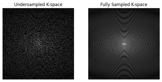
3. Apply the Sampling Mask to Create Undersampled k-space by famc#
undersampled_kspace = bart(1, 'fmac', fully_sampled_kspace, sampling_mask)
# Visualizing the images using Matplotlib
fig, axes = plt.subplots(1, 2, figsize=(8, 4))

# Plot undersampled k-space
axes[0].imshow((abs(undersampled_kspace)**0.3), cmap='gray')
axes[0].set_title('Undersampled K-space')
axes[0].axis('off')  # Hide axes

# Plot fully sampled k-space
axes[1].imshow((abs(fully_sampled_kspace)**0.3), cmap='gray')
axes[1].set_title('Fully Sampled K-space')
axes[1].axis('off')  # Hide axes

plt.show()
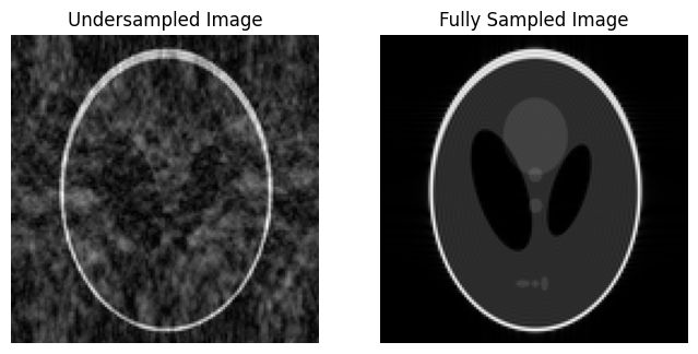
4. Computes the inverse Fourier transform of the k-space data to obtain the image by fft#
-i: Computes the inverse Fourier transform
-u: Unitary inverse Fourier transform
3: Corresponds to the first two dimensions
fully_sampled_image = bart(1, 'fft -i -u 3', fully_sampled_kspace)
undersampled_image = bart(1, 'fft -i -u 3', undersampled_kspace)
# Visualizing the images using Matplotlib
fig, axes = plt.subplots(1, 2, figsize=(8, 4))

# Plot undersampled image
axes[0].imshow((abs(undersampled_image)), cmap='gray')
axes[0].set_title('Undersampled Image')
axes[0].axis('off')  # Hide axes

# Plot fully sampled image
axes[1].imshow((abs(fully_sampled_image)), cmap='gray')
axes[1].set_title('Fully Sampled Image')
axes[1].axis('off')  # Hide axes

plt.show()
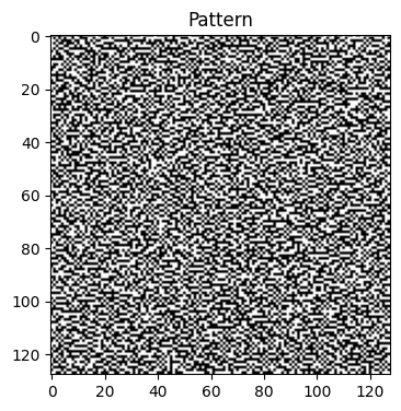
Example#
pattern = bart(1, 'pattern', undersampled_kspace).real
# Visualizing the images using Matplotlib
plt.figure(figsize=(4,6))
plt.imshow((abs(pattern)**.3), cmap='gray')
plt.title('Pattern')
plt.show()