bart fmac

=================================================================================================================

The bart fmac command in BART performs element-wise multiplication and summation over specified dimensions, which is particularly useful for operations like applying coil sensitivity maps to k-space data.

Where we can view the full usage string and optional arguments with the -h flag.

!bart fmac -h

Usage: fmac [-A] [-C] [-s d] <input1> [<input2>] <output> 

Multiply <input1> and <input2> and accumulate in <output>.
If <input2> is not specified, assume all-ones.

-A      add to existing output (instead of overwriting)
-C      conjugate input2
-s b    squash dimensions selected by bitmask b
-h      help

How bart fmac work

Element-wise Multiplication

When both input tensors A and B have the same dimensions, fmac performs element-wise multiplication:

\[ O_{m,n} = A_{m,n} \cdot B_{m,n} \]

Example:

Given two matrices:

\[\begin{split} A = \begin{bmatrix} a_{11} & a_{12} \\ a_{21} & a_{22} \end{bmatrix}, \quad B = \begin{bmatrix} b_{11} & b_{12} \\ b_{21} & b_{22} \end{bmatrix} \end{split}\]

The element-wise multiplication produces:

\[\begin{split} O = A \circ B = \begin{bmatrix} a_{11} \cdot b_{11} & a_{12} \cdot b_{12} \\ a_{21} \cdot b_{21} & a_{22} \cdot b_{22} \end{bmatrix} \end{split}\]

s: Squashing a Dimension

If we squash the first dimension (b = 1 in binary: 0001), fmac sums over rows:

\[ O = \sum_{\text{rows}} (A \circ B) \]

\[ O = \begin{bmatrix} (a_{11} \cdot b_{11}) + (a_{21} \cdot b_{21}) & (a_{12} \cdot b_{12}) + (a_{22} \cdot b_{22}) \end{bmatrix} \]

Squashing the Second Dimension (-s 2)

If we squash the second dimension (b = 2 in binary: 0010), fmac sums over columns:

\[ O = \sum_{\text{columns}} (A \circ B) \]

\[\begin{split} O = \begin{bmatrix} (a_{11} \cdot b_{11}) + (a_{12} \cdot b_{12}) \\ (a_{21} \cdot b_{21}) + (a_{22} \cdot b_{22}) \end{bmatrix} \end{split}\]

This results in a 1D column vector:

Full Summation (-s 3)

If b = 3 (binary 0011), it squashes both dimensions, resulting in a single scalar:

\[ O = (a_{11} \cdot b_{11}) + (a_{12} \cdot b_{12}) + (a_{21} \cdot b_{21}) + (a_{22} \cdot b_{22}) \]

For Mismatched Dimensions with Singleton dimension

If B has a singleton dimension (one column instead of two), fmac will loop over the missing dimension:

\[\begin{split} A = \begin{bmatrix} a_{11} & a_{12} \\ a_{21} & a_{22} \end{bmatrix}, \quad B = \begin{bmatrix} b_{11} \\ b_{21} \end{bmatrix} \end{split}\]

Since B has only one column,

\[\begin{split} O = A \circ B = \begin{bmatrix} a_{11} \cdot b_{11} & a_{12} \cdot b_{11} \\ a_{21} \cdot b_{21} & a_{22} \cdot b_{21} \end{bmatrix} \end{split}\]

Summary of Broadcasting Rule

• If a dimension in B is 1, fmac copies its values across that dimension.

• If A and B have different dimensions that are not 1, fmac throws an error.

Example for Matrix (using Bash)

Create a Matrix (A), Dimension as 2 x 2 x 2

!bart vec $(seq 1 8) array_A # Generate a array with values from 1 to 8 

!bart reshape $(bart bitmask 0 1 2) 2 2 2 array_A matrix_A # Reshape the array to Dimension as 2 x 2 x 2

!bart show matrix_A

+1.000000e+00+0.000000e+00i	+2.000000e+00+0.000000e+00i
+3.000000e+00+0.000000e+00i	+4.000000e+00+0.000000e+00i
+5.000000e+00+0.000000e+00i	+6.000000e+00+0.000000e+00i
+7.000000e+00+0.000000e+00i	+8.000000e+00+0.000000e+00i

Create a Matrix (B), Dimension as 2 x 2 x 2

!bart vec $(seq 2 9) array_B # Generate a array with values from 2 to 9 

!bart reshape $(bart bitmask 0 1 2) 2 2 2 array_B matrix_B # Reshape the array to Dimension as 2 x 2 x 2

!bart show matrix_B

+2.000000e+00+0.000000e+00i	+3.000000e+00+0.000000e+00i
+4.000000e+00+0.000000e+00i	+5.000000e+00+0.000000e+00i
+6.000000e+00+0.000000e+00i	+7.000000e+00+0.000000e+00i
+8.000000e+00+0.000000e+00i	+9.000000e+00+0.000000e+00i

Example 1.1:

Performs element-wise multiplication of matrix_A and matrix_B and stores the result in matrix_output

!bart fmac matrix_A matrix_B matrix_output

!bart show matrix_output

+2.000000e+00+0.000000e+00i	+6.000000e+00+0.000000e+00i
+1.200000e+01+0.000000e+00i	+2.000000e+01+0.000000e+00i
+3.000000e+01+0.000000e+00i	+4.200000e+01+0.000000e+00i
+5.600000e+01+0.000000e+00i	+7.200000e+01+0.000000e+00i

-A: Adds the computed result to an existing output file instead of overwriting it

Mathematical Representation

Without -A:

\[ O = A \cdot B \]

With -A:

\[ O = O_{\text{existing}} + (A \cdot B) \]

where the previous values in \(O_{\text{existing}}\) are updated by adding the new computation.

Example 1.2:

Performs element-wise multiplication of matrix_A and matrix_B, and then adds the result to matrix_output for Example 1.1 instead of overwriting it.

!bart fmac -A matrix_A matrix_B matrix_output

!bart show matrix_output

+4.000000e+00+0.000000e+00i	+1.200000e+01+0.000000e+00i
+2.400000e+01+0.000000e+00i	+4.000000e+01+0.000000e+00i
+6.000000e+01+0.000000e+00i	+8.400000e+01+0.000000e+00i
+1.120000e+02+0.000000e+00i	+1.440000e+02+0.000000e+00i

-C: Takes the complex conjugate of the second input (input2) before performing the element-wise multiplication.

Given two matrices:

\[\begin{split} A = \begin{bmatrix} a_{11} & a_{12} \\ a_{21} & a_{22} \end{bmatrix}, \quad B = \begin{bmatrix} b_{11} & b_{12} \\ b_{21} & b_{22} \end{bmatrix} \end{split}\]

The element-wise multiplication produces:

\[\begin{split} O = A \circ B = \begin{bmatrix} a_{11} \cdot b_{11} & a_{12} \cdot b_{12} \\ a_{21} \cdot b_{21} & a_{22} \cdot b_{22} \end{bmatrix} \end{split}\]

Using -C for Complex Conjugation

When using the -C option, the second input matrix B is conjugated before multiplication:

\[ O = A \cdot B^* \]

where the complex conjugate of \(B\) is:

\[\begin{split} B^* = \begin{bmatrix} {b_{11}}^* & {b_{12}}^* \\ {b_{21}}^* & {b_{22}}^* \end{bmatrix} \end{split}\]

Example 1.3:

Performs element-wise multiplication of matrix_A with the complex conjugate of matrix_C, and stores the result in matrix_output_conjugate.

!bart vec 1+1i 2+2i matrix_C # Generate a matrix with Dimension as 2 x 1

!bart show matrix_C

+1.000000e+00+1.000000e+00i	+2.000000e+00+2.000000e+00i

!bart fmac -C matrix_A matrix_C matrix_output_conjugate

!bart show matrix_output_conjugate

+1.000000e+00-1.000000e+00i	+4.000000e+00-4.000000e+00i
+3.000000e+00-3.000000e+00i	+8.000000e+00-8.000000e+00i
+5.000000e+00-5.000000e+00i	+1.200000e+01-1.200000e+01i
+7.000000e+00-7.000000e+00i	+1.600000e+01-1.600000e+01i

!bart show -m matrix_output_conjugate

Type: complex float
Dimensions: 16
AoD:	2	2	2	1	1	1	1	1	1	1	1	1	1	1	1	1

Note: As the example showing, if the dimensions of matrix_A and matrix_C do not match, and matrix_C with Singleton dimension. BART will repeat the elements of matrix_C along the mismatched dimension to match matrix_A. As shown in the example, the matrix_C (2×1) is repeated to perform element-wise multiplication with matrix_A.

-s b: Squashes dimensions (summed along the dimensions) specified by the bitmask b after performing element-wise multiplication.

Example 1.4:

Performs element-wise multiplication and sums over the first dimension.

!bart fmac -s 1 matrix_A matrix_B matrix_output_squash1

!bart show matrix_output

+4.000000e+00+0.000000e+00i	+1.200000e+01+0.000000e+00i
+2.400000e+01+0.000000e+00i	+4.000000e+01+0.000000e+00i
+6.000000e+01+0.000000e+00i	+8.400000e+01+0.000000e+00i
+1.120000e+02+0.000000e+00i	+1.440000e+02+0.000000e+00i

!bart show matrix_output_squash1

+8.000000e+00+0.000000e+00i	+3.200000e+01+0.000000e+00i
+7.200000e+01+0.000000e+00i	+1.280000e+02+0.000000e+00i

Example 1.5:

Performs element-wise multiplication and sums over the all the dimensions.

!bart fmac -s 7 matrix_A matrix_B matrix_output_squash2

!bart show matrix_output_squash2

+2.400000e+02+0.000000e+00i

Example Workflow for MRI (python)

# Importing the required libraries
import numpy as np
import matplotlib.pyplot as plt
%matplotlib inline

import cfl
from bart import bart

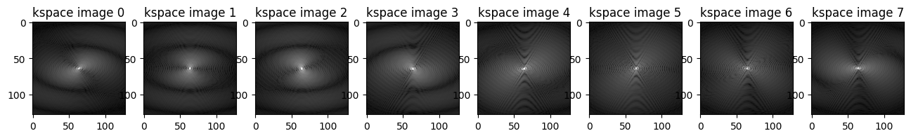
1. Generate Phantom in k-Space Directly

Generate Shepp-Logan phantom directly in k-space:

ksp = bart(1, 'phantom -x 128 -k -s 8')

# Visualizing the images using Matplotlib 
plt.figure(figsize=(16,20))
for i in range(8):
    plt.subplot(1, 8, i+1)
    plt.imshow(abs(ksp[...,i])**.3, cmap='gray')
    plt.title('kspace image {}'.format(i))

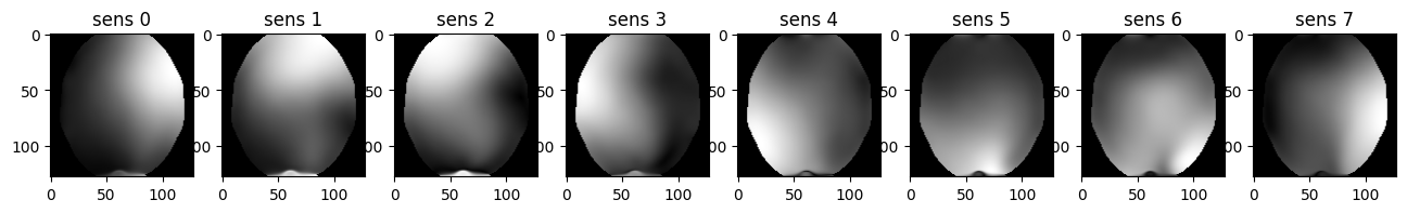
2. Generate Sensitivity Maps

Create sensitivity maps for 8 coils:

-m 1: Compute one set of sensitivity maps.

sens = bart(1, 'ecalib -m 1', ksp)

Done.

sens.shape

(128, 128, 1, 8)

# Visualizing the sensitivity maps using Matplotlib 
plt.figure(figsize=(16,20))
for i in range(8):
    plt.subplot(1, 8, i+1)
    plt.imshow(abs(sens[...,i]), cmap='gray')
    plt.title('sens {}'.format(i))

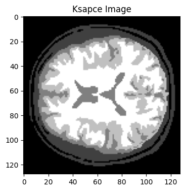
3. Generate a Brain Image by phantom

brain = bart(1, 'phantom --BRAIN -x 128')

# Visualizing the image using Matplotlib
plt.figure(figsize=(4, 6))
plt.imshow(np.abs(brain), cmap='gray')
plt.title('Ksapce Image')

Text(0.5, 1.0, 'Ksapce Image')

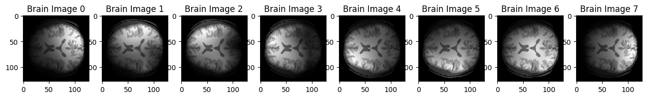
Example 2.1: Use bart fmac to apply sensitivity maps to the brain image:

brain_fmac = bart(1, 'fmac', brain, sens)

# Visualizing the images using Matplotlib 
plt.figure(figsize=(16,20))
for i in range(8):
    plt.subplot(1, 8, i+1)
    plt.imshow(abs(brain_fmac[...,i]), cmap='gray')
    plt.title('Brain Image {}'.format(i))

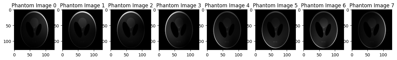
Performing an inverse FFT on k-space data (ksp)

phantom = bart(1, 'fft -i 3', ksp)

# Visualizing the images using Matplotlib 
plt.figure(figsize=(16,20))
for i in range(8):
    plt.subplot(1, 8, i+1)
    plt.imshow(abs(phantom[...,i]), cmap='gray')
    plt.title('Phantom Image {}'.format(i))

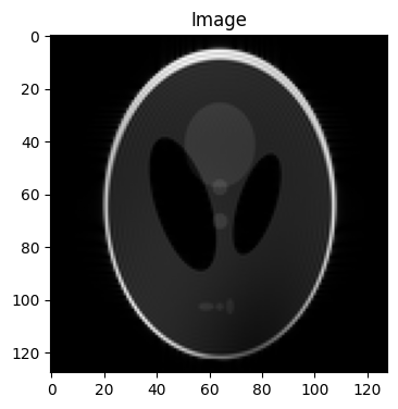
Example 2.2: Performing coil combination using sensitivity maps (sens) to obtain a final image.

-C: Uses the conjugate of sens.

-s 8: Squashes dimension 8 (typically the coil dimension in BART).

image = bart(1, 'fmac -C -s 8', phantom, sens)

# Visualizing the image using Matplotlib
plt.figure(figsize=(4, 6))
plt.imshow(np.abs(image), cmap='gray')
plt.title('Image')

Text(0.5, 1.0, 'Image')