bart fft

`bart fft`#

=================================================================================================================

The bart fft command in BART command performs a Fast Fourier Transform (FFT) along selected dimensions of input data.

Where we can view the full usage string and optional arguments with the -h flag.

!bart fft -h

Usage: fft [-u] [-i] [-n] bitmask <input> <output> 

Performs a fast Fourier transform (FFT) along selected dimensions.

-u    unitary
-i    inverse
-n    un-centered
-h    help

Mathematical Formulation#

Standard Forward FFT#

For an input signal \(x(n)\), the discrete Fourier transform (DFT) is:

\[ X(k) = \sum_{n=0}^{N-1} x(n) e^{-j 2\pi kn / N} \]

where:

\(x(n)\) is the input data.
\(X(k)\) is the FFT output.
\(N\) is the length of the transformed dimension.

Inverse FFT (`-i` Option)#

The inverse FFT (IFFT) transforms frequency-domain data back into the time/spatial domain:

\[ x(n) = \frac{1}{N} \sum_{k=0}^{N-1} X(k)e^{j 2\pi kn / N} \]

Applying bart fft -i computes this inverse transform.

k-space to Image Domain: In MRI, data is initially acquired in k-space, which is the spatial frequency domain. To reconstruct an image, an inverse FFT is typically applied to the k-space data to transform it into the image domain.

Unitary FFT (`-u` Option)#

By default, the FFT scales the transformed values by N. The unitary FFT normalizes the result:

\[ X_u(k) = \frac{1}{\sqrt{N}} \sum_{n=0}^{N-1} x(n)e^{-j 2\pi kn / N} \]

which ensures that applying fft followed by ifft returns the original signal without scaling.

Uncentered FFT (`-n` Option)#

The uncentered FFT (-n) performs a Fast Fourier Transform without shifting the zero-frequency (DC) component to the center. In standard FFT implementations, the output is usually shifted so that the low frequencies (including DC) are centered in k-space. Using -n keeps the DC component at its original location.

The frequency indices in the uncentered FFT (-n) are assigned sequentially:

\[ X_{\text{uncentered}}(k) = \sum_{n=0}^{N-1} x(n)e^{-j 2\pi kn / N}, \quad k = 0, 1, 2, ..., N - 1 \]

Mathematical Interpretation of the Shift#

The FFT shift operation is mathematically represented by multiplying the input signal by a phase term:

\[ x_{\text{shifted}}(n) = x(n) \cdot (-1)^n \]

This results in a frequency-domain shift:

\[ X_{\text{shifted}}(k) = X \left( (k + N/2) \mod N \right) \]

Examples for 1D Array (Using Bash)#

FFT Numerical Comparison Chart#

Index	Original Signal (x)	Standard FFT (X_fft)	Unitary FFT (X_fft_u)	Uncentered FFT (X_fft_n)
0	1.0	(-2 + 0j)	(-1 + 0j)	(10 + 0j)
1	2.0	(2 + 2j)	(1 + 1j)	(-2 + 2j)
2	3.0	(10 + 0j)	(5 + 0j)	(-2 + 0j)
3	4.0	(2 - 2j)	(1 - 1j)	(-2 - 2j)

Creates a 1D vector in BART and stores it in the variable `x`.#

!bart vec 1 2 3 4 x

!bart show x

+1.000000e+00+0.000000e+00i	+2.000000e+00+0.000000e+00i	+3.000000e+00+0.000000e+00i	+4.000000e+00+0.000000e+00i

Example 1: Performs a Fast Fourier Transform (FFT) along the first dimension of the vector `x` and stores the output in `X_fft`.#

!bart fft 1 x X_fft

!bart show X_fft

-2.000000e+00+0.000000e+00i	+2.000000e+00+2.000000e+00i	+1.000000e+01-0.000000e+00i	+2.000000e+00-2.000000e+00i

Example 2: Performs a unitary Fast Fourier Transform (FFT) along the first dimension of the vector and stores the output in `X_fft_u`#

!bart fft -u 1 x X_fft_u

!bart show X_fft_u

-1.000000e+00+0.000000e+00i	+1.000000e+00+1.000000e+00i	+5.000000e+00-0.000000e+00i	+1.000000e+00-1.000000e+00i

Example 3: Performs a uncentered FFT along the first dimension of the vector and stores the output in `X_fft_n`#

!bart fft -n 1 x X_fft_n

!bart show X_fft_n

+1.000000e+01+0.000000e+00i	-2.000000e+00+2.000000e+00i	-2.000000e+00+0.000000e+00i	-2.000000e+00-2.000000e+00i

Examples for image(Using Python)#

# Importing the required libraries
import numpy as np
import matplotlib.pyplot as plt
%matplotlib inline

import cfl
from bart import bart

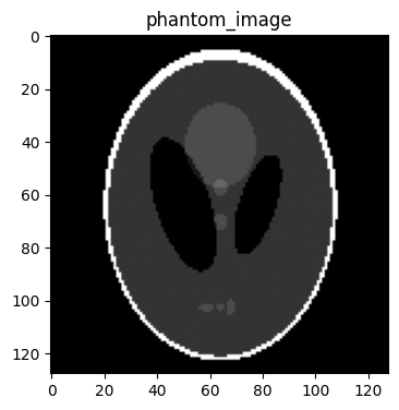
phantom_image = bart(1, 'phantom -x 128') # Generate a phantom image with size 128x128

# Visualizing the image using Matplotlib
plt.figure(figsize=(4,6))
plt.imshow(abs(phantom_image), cmap='gray')
plt.title('phantom_image')

Text(0.5, 1.0, 'phantom_image')

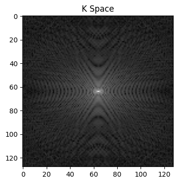
_images/c40b662976cd6b9b2d96e0e61474115ce5702487f482cb35f255110ead564031.png

Exmaple 4: Applying FFT along the first and second dimensions (transform from image domain to k-sapce data).#

kspace = bart(1, 'fft 3', phantom_image)

# Visualizing the image using Matplotlib
plt.figure(figsize=(4,6))
plt.imshow(abs(kspace)**.3, cmap='gray')
plt.title('K Space')

Text(0.5, 1.0, 'K Space')

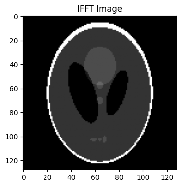
_images/b2123834916b264291ec3e49eeaa3522ad5097c2f7432316625e9b43fd2b01b0.png

Exmaple 5: Applying inverse FFT along the first and second dimensions (transform from k-space data to image domain).#

By -i

image = bart(1, 'fft -i 3', kspace)

# Visualizing the image using Matplotlib
plt.figure(figsize=(4,6))
plt.imshow(abs(image), cmap='gray')
plt.title('IFFT Image')

Text(0.5, 1.0, 'IFFT Image')

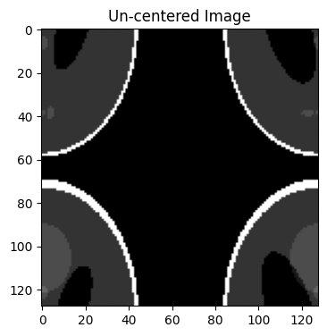
_images/1430d6e9434924434602ffe997016954bc05bf9748240cc0499cd2dc089fac18.png

Exmaple 6: Applying un-centered IFFT along the first and second dimensions.#

By -in

image_n = bart(1, 'fft -in 3', kspace)

# Visualizing the image using Matplotlib
plt.figure(figsize=(4,6))
plt.imshow(abs(image_n), cmap='gray')
plt.title('Un-centered Image')

Text(0.5, 1.0, 'Un-centered Image')

_images/e50812bf77446626b59f406c1667923d376a4b3bfacf8dc2f17231ed167d4d79.png

bart fft

Contents

bart fft#