bart homodyne

=================================================================================================================

The bart homodyne command performs homodyne reconstruction along a specified dimension of k-space data. Homodyne reconstruction is a technique used in partial Fourier imaging to reconstruct images from asymmetric k-space data by estimating the missing phase information. And can take optional arguments like a phase reference and an offset ramp filter. It can also save some operations if the data are already Fourier transformed or uncentered

Where we can view the full usage string and optional arguments with the -h flag.

!bart homodyne -h

Usage: homodyne [-r f] [-I] [-C] [-P <file>] [-n] dim fraction <input> <output> 

Perform homodyne reconstruction along dimension dim.

-r alpha         Offset of ramp filter, between 0 and 1. alpha=0 is a full ramp, alpha=1 is a horizontal line
-I               Input is in image domain
-C               Clear unacquired portion of kspace
-P phase_ref>    Use <phase_ref> as phase reference
-n               use uncentered ffts
-h               help

Where:

dim: The dimension along which homodyne reconstruction is performed.

fraction: The fraction of k-space that has been acquired. Typically, values are between 0 and 1, where 1 means full k-space data is available, and lower values indicate partial Fourier acquisitions.

<input>: The input file (k-space data).

<output>: The output file (reconstructed image).

Example Workflow (using python)

# Importing the required libraries
import numpy as np
import matplotlib.pyplot as plt
%matplotlib inline

import cfl
from bart import bart

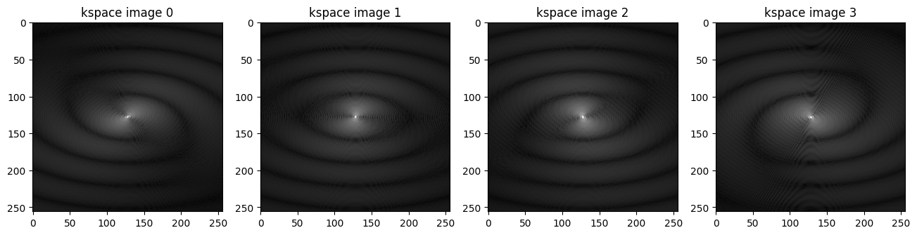
Generate a multi-coil image in k-space using the phantom simulation tool

ksp_full = bart(1, 'phantom -k -s 4 -x 256')

# Visualizing the multi-coil kspace images using Matplotlib 
plt.figure(figsize=(16,20))
for i in range(4):
    plt.subplot(1, 4, i+1)
    plt.imshow(np.abs(ksp_full[...,i])**0.3, cmap='gray')
    plt.title('kspace image {}'.format(i))

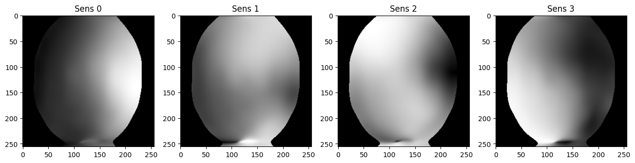
Compute coil sensitivity maps from fully sampled k-space data by ecalib

sens = bart(1, 'ecalib -m 1', ksp_full)

Done.

# Visualizing the multi-coil kspace images using Matplotlib 
plt.figure(figsize=(16,20))
for i in range(4):
    plt.subplot(1, 4, i+1)
    plt.imshow(np.abs(sens[...,i]), cmap='gray')
    plt.title('Sens {}'.format(i))

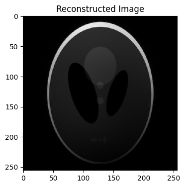
Performs parallel imaging reconstruction using pics

-S re-scale the image after reconstruction

reco_full = bart(1, 'pics -S', ksp_full, sens) 

Size: 65536 Samples: 65536 Acc: 1.00
Regularization terms: 0, Supporting variables: 0
conjugate gradients
Total Time: 0.066936

# Visualizing the image using Matplotlib
plt.figure(figsize=(4, 6))
plt.imshow(abs(reco_full), cmap='gray')
plt.title('Reconstructed Image')

Text(0.5, 1.0, 'Reconstructed Image')

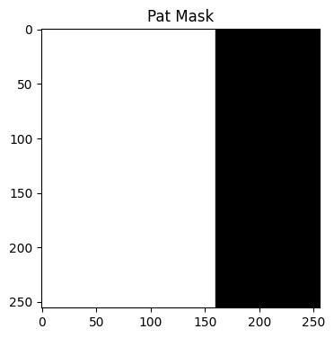
Creates a binary mask (pat)

Generates a 2D 256 × 256 matrix filled with ones (p1).

p1 = bart(1, 'ones 2 256 256')

Reduces the size of the second dimension from 256 to 160 by bart resize

p2 = bart(1, 'resize 1 160', p1)

Resizing back to 256 fills the missing 96 rows with zeros.

pat = bart(1, 'resize 1 256', p2)

# Visualizing the image using Matplotlib
plt.figure(figsize=(4, 6))
plt.imshow(abs(pat), cmap='gray')
plt.title('Pat Mask')

Text(0.5, 1.0, 'Pat Mask')

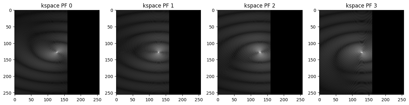
Performs element-wise multiplication of the fully sampled k-space (ksp_full) with the partial Fourier mask (pat).

ksp_pf = bart(1, 'fmac', ksp_full, pat) 

# Visualizing the multi-coil kspace images using Matplotlib 
plt.figure(figsize=(16,20))
for i in range(4):
    plt.subplot(1, 4, i+1)
    plt.imshow(np.abs(ksp_pf[...,i])**.3, cmap='gray')
    plt.title('kspace PF {}'.format(i))

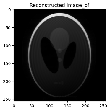
Performs parallel imaging reconstruction on the partially acquired k-space

reco_pf = bart(1, 'pics -S', ksp_pf, sens)

Size: 65536 Samples: 40960 Acc: 1.60
Regularization terms: 0, Supporting variables: 0
conjugate gradients

Total Time: 0.209182

# Visualizing the image using Matplotlib
plt.figure(figsize=(4, 6))
plt.imshow(abs(reco_pf), cmap='gray')
plt.title('Reconstructed Image_pf')

Text(0.5, 1.0, 'Reconstructed Image_pf')

Multiplies the reconstructed image (reco_pf) with the coil sensitivity maps (sens), converting the combined image back into individual coil images.

reco_pf_cimgs = bart(1, 'fmac', reco_pf, sens)

# Visualizing the multi-coil kspace images using Matplotlib 
plt.figure(figsize=(16,20))
for i in range(4):
    plt.subplot(1, 4, i+1)
    plt.imshow(np.abs(reco_pf_cimgs[...,i]), cmap='gray')
    plt.title('Coil Image {}'.format(i))

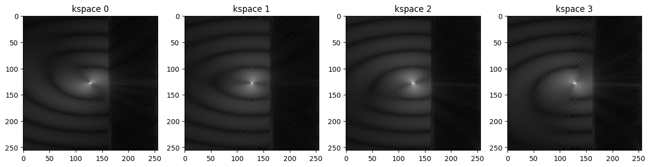
Applies the Fourier Transform (FFT) to convert the coil images (reco_pf_cimgs) back to k-space (reco_pf_ksp)

reco_pf_ksp = bart(1, 'fft -u 7', reco_pf_cimgs)

# Visualizing the multi-coil kspace images using Matplotlib 
plt.figure(figsize=(16,20))
for i in range(4):
    plt.subplot(1, 4, i+1)
    plt.imshow(np.abs(reco_pf_ksp[...,i])**.3, cmap='gray')
    plt.title('kspace {}'.format(i))

Example 1

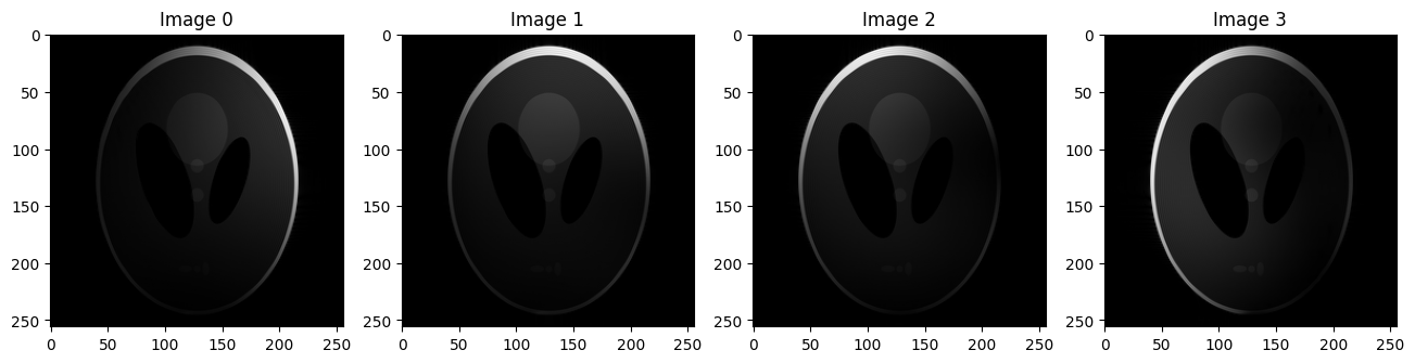
Performs homodyne reconstruction on the coil images (reco_pf_cimgs), correcting the missing phase information due to partial Fourier acquisition.

-C: Clears the unacquired portion of k-space before reconstruction.

-I: Indicates that the input (reco_pf_cimgs) is in the image domain.

1: Specifies the phase encoding dimension (Dimension 1).

.625: Fraction of acquired k-space (160/256 = 62.5%).

reco_pf_cimgs_hd = bart(1, 'homodyne -C -I 1 .625', reco_pf_cimgs)

# Visualizing the multi-coil kspace images using Matplotlib 
plt.figure(figsize=(16,20))
for i in range(4):
    plt.subplot(1, 4, i+1)
    plt.imshow(np.abs(reco_pf_cimgs_hd[...,i]), cmap='gray')
    plt.title('Reco_coil_image {}'.format(i))

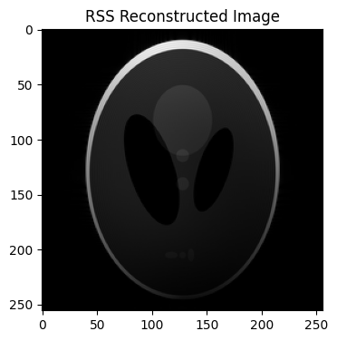
Combines the homodyne-corrected coil images (reco_pf_cimgs_hd) into a final reconstructed magnitude image using the root-sum-of-squares (RSS) method.

reco_pf_hd = bart(1, 'rss 8', reco_pf_cimgs_hd) # 8 Specifies the coil dimension

# Visualizing the image using Matplotlib
plt.figure(figsize=(4, 6))
plt.imshow(abs(reco_pf_hd), cmap='gray')
plt.title('RSS Reconstructed Image')

Text(0.5, 1.0, 'RSS Reconstructed Image')

Example 2: We could also use homodyne on k-space. The result will be the same

-C: Clears the unacquired portion of k-space before reconstruction.

1: Specifies the phase encoding dimension (Dimension 1).

.625: Fraction of acquired k-space (160/256 = 62.5%).

reco_pf_cimgs_hd2 = bart(1, 'homodyne -C 1 .625', reco_pf_ksp)

# Visualizing the multi-coil kspace images using Matplotlib 
plt.figure(figsize=(16,20))
for i in range(4):
    plt.subplot(1, 4, i+1)
    plt.imshow(np.abs(reco_pf_cimgs_hd2[...,i]), cmap='gray')
    plt.title('Image {}'.format(i))

Compute the Normalized Root Mean Square Error (NRMSE) between reco_pf_cimgs_hd and reco_pf_cimgs_hd2

nrmse = np.linalg.norm(reco_pf_cimgs_hd2 - reco_pf_cimgs_hd) / np.linalg.norm(reco_pf_cimgs_hd)
print("NRMSE:", nrmse)

NRMSE: 0.0

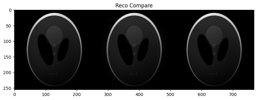
Combine multiple reconstructed images along a specified dimension

reco_compare = bart(1, 'join 1', reco_full, reco_pf, reco_pf_hd)

# Visualizing the image using Matplotlib
plt.figure(figsize=(10, 10))
plt.imshow(abs(reco_compare), cmap='gray')
plt.title('Reco Compare')

Text(0.5, 1.0, 'Reco Compare')

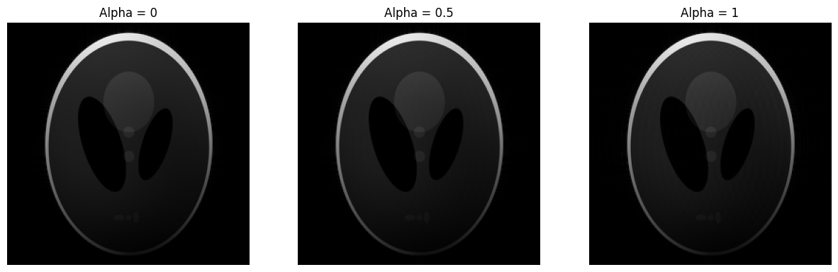
-r alpha Option in bart homodyne

Example 3

The -r option in the bart homodyne command controls the shape of the ramp filter used in homodyne reconstruction. The ramp filter determines how much smoothing is applied to k-space before phase correction.

-r 0 (default): Use when strong phase correction is needed.

-r 0.5: Balanced smoothing & detail retention.

-r 1: Use when minimal smoothing is needed but can lead to incomplete phase correction.

reco_pf_cimgs_hd_0 = bart(1, 'homodyne -r 0 -C -I 1 .625', reco_pf_cimgs)
reco_pf_hd_0 = bart(1, 'rss 8', reco_pf_cimgs_hd_0)

reco_pf_cimgs_hd_05 = bart(1, 'homodyne -r 0.5 -C -I 1 .625', reco_pf_cimgs)
reco_pf_hd_05 = bart(1, 'rss 8', reco_pf_cimgs_hd_05)

reco_pf_cimgs_hd_1 = bart(1, 'homodyne -r 1 -C -I 1 .625', reco_pf_cimgs)
reco_pf_hd_1 = bart(1, 'rss 8', reco_pf_cimgs_hd_1)

reco_alpha_compare = bart(1, 'join 1', reco_pf_hd_0, reco_pf_hd_05, reco_pf_hd_1)

# Visualizing the images using Matplotlib
fig, axes = plt.subplots(1, 3, figsize=(15, 10))

axes[0].imshow((abs(reco_pf_hd_0)), cmap='gray')
axes[0].set_title('Alpha = 0')
axes[0].axis('off')  # Hide axes

axes[1].imshow((abs(reco_pf_hd_05)), cmap='gray')
axes[1].set_title('Alpha = 0.5')
axes[1].axis('off')  # Hide axes

axes[2].imshow((abs(reco_pf_hd_1)), cmap='gray')
axes[2].set_title('Alpha = 1')
axes[2].axis('off')  # Hide axes

plt.show()