bart caldir#
============================================================================================================
The bart caldir command in BART is used to estimate coil sensitivities from the k-space center of MRI data, which is generally a fully sampled area of the MRI data. This method is based on the approach by McKenzie et al. [1], which uses a direct estimation technique to determine coil sensitivity profiles. The calibration region’s size is automatically determined but limited by the {cal_size} parameter specified by the user.
[1] McKenzie CA, Yeh EN, Ohliger MA, Price MD, Sodickson DK. Self-calibrating parallel imaging with automatic coil sensitivity extraction. Magn Reson Med 2002; 47:529-538.
Where we can view the full usage string and optional arguments with the -h flag.
!bart caldir -h
Usage: caldir cal_size <input> <output>

Estimates coil sensitivities from the k-space center using
a direct method (McKenzie et al.). The size of the fully-sampled
calibration region is automatically determined but limited by
{cal_size} (e.g. in the readout direction).

-h  help
Parameters#
cal_size: Specifies the maximum size of the fully-sampled calibration region, typically in the readout direction.<input>: The input file, which is usually a k-space data file.<output>: The output file where the estimated coil sensitivities will be stored.-h: Displays help information.
Example 1: Estimates Coil Sensitivities Small cal_size (Using Python)#
# Importing the required libraries
import numpy as np
import matplotlib.pyplot as plt
%matplotlib inline

import cfl
from bart import bart
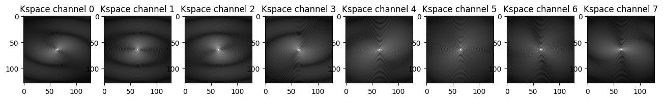
Generate a multi-coil image in k-space using the phantom simulation tool#
multi_coil_kspace = bart(1, 'phantom -x 128 -k -s 8')
# Visualizing the multi-coil kspace data using Matplotlib
plt.figure(figsize=(16,20))
for i in range(8):
    plt.subplot(1, 8, i+1)
    plt.imshow(abs(multi_coil_kspace[...,i])**.3, cmap='gray')
    plt.title('Kspace channel {}'.format(i))
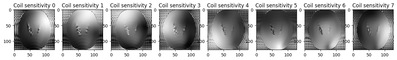
Estimated the coil sensitivity by using caldir with cal_size = 6#
coil_sen = bart(1, 'caldir 6', multi_coil_kspace)
Calibration region 6x6x1
Done.
# Visualizing the images using Matplotlib
plt.figure(figsize=(16,20))
for i in range(8):
    plt.subplot(1, 8, i+1)
    plt.imshow(abs(coil_sen[...,i]), cmap='gray')
    plt.title('Coil sensitivity {}'.format(i))
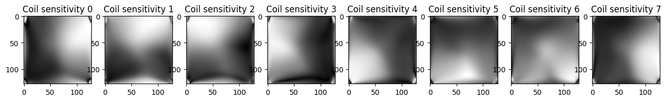
Example 2: Estimates Coil Sensitivities with Large cal_size (Using Python)#
Estimated the coil sensitivity by using caldir with “cal_size = 24”#
coil_sen_1 = bart(1, 'caldir 24', multi_coil_kspace)
Calibration region 24x24x1
Done.
# Visualizing the images using Matplotlib
plt.figure(figsize=(16,20))
for i in range(8):
    plt.subplot(1, 8, i+1)
    plt.imshow(abs(coil_sen_1[...,i]), cmap='gray')
    plt.title('Coil sensitivity {}'.format(i))