bart phantom#
===========================================================================================================
The bart phantom command in BART is used to generate synthetic MRI phantoms in both image and k-space domains.
Where we can view the full usage string and optional arguments with the -h flag.
!bart phantom -h
Usage: phantom [-s d] [-S d] [-k] [-t <file>] [-G] [-T] [--NIST] [--SONAR] [--BRAIN] [--ELLIPSOID] [--ellipsoid_center d:d:d] [--ellipsoid_axes f:f:f] [-N d] [-B] [--FILE <file>] [-x d] [-g d] [-3] [-b] [-r d] [--rotation-angle f] [--rotation-steps d] [--coil ...] <output>

Image and k-space domain phantoms.

-s nc                       nc sensitivities
-S nc                       Output nc sensitivities
-k                          k-space
-t file                     trajectory
-G                          geometric object phantom
-T                          tubes phantom
--NIST                      NIST phantom (T2 sphere)
--SONAR                     Diagnostic Sonar phantom
--BRAIN                     BRAIN geometry phantom
--ELLIPSOID                 Ellipsoid.
--ellipsoid_center d:d:d    x,y,z center coordinates of ellipsoid.
--ellipsoid_axes f:f:f      Axes lengths of ellipsoid.
-N num                      Random tubes phantom with num tubes
-B                          BART logo
--FILE name                 Arbitrary geometry based on multicfl file.
-x n                        dimensions in y and z
-g n=1,2,3                  select geometry for object phantom
-3                          3D
-b                          basis functions for geometry
-r seed                     random seed initialization
--rotation-angle [deg]      Angle of rotation
--rotation-steps n          Number of rotation steps
--coil ...                  configure type of coil
-h                          help
Examples (Using Python)#
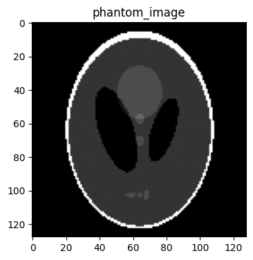
Example 1: Generating a Phantom in Image Space#
This example generates a phantom in image space.#
# Importing the required libraries
import numpy as np
import matplotlib.pyplot as plt
%matplotlib inline

import cfl
from bart import bart
phantom_image = bart(1, 'phantom -x 128') # Generate a phantom image with size 128x128
# Visualizing the image using Matplotlib
plt.figure(figsize=(4,6))
plt.imshow(abs(phantom_image), cmap='gray')
plt.title('phantom_image')
Text(0.5, 1.0, 'phantom_image')
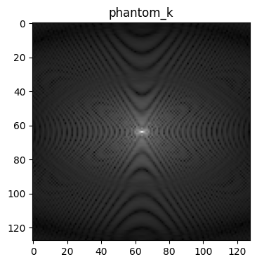
Example 2: Generating a Phantom in k-Space#
This example generates a phantom in k-space by using -k.#
phantom_k = bart(1, 'phantom -x 128 -k') # Generate a phantom image in k-space with size 128x128
# Visualizing the image using Matplotlib
plt.figure(figsize=(4,6))
plt.imshow(abs(phantom_k)**.3, cmap='gray')
plt.title('phantom_k')
Text(0.5, 1.0, 'phantom_k')
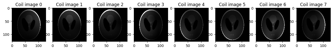
Example 3: Generate a multi-coil image using the phantom simulation tool in BART#
Generate a multi-coil image with size 128x128 and 8 coils by using -s.#
multi_coil_image = bart(1, 'phantom -x 128 -s 8') # Generate a multi-coil image with size 128x128 and 8 coils
# Visualizing the multi-coil images using Matplotlib
plt.figure(figsize=(16,20))
for i in range(8):
    plt.subplot(1, 8, i+1)
    plt.imshow(abs(multi_coil_image[...,i]), cmap='gray')
    plt.title('Coil image {}'.format(i))
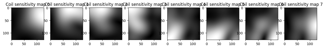
Output the sensitivity maps directly with -S.#
sens_maps = bart(1, 'phantom -x 128 -S 8') # Generate the maps corresponding to a multi-coil image with size 128x128 and 8 coils
# Visualizing the multi-coil images using Matplotlib
plt.figure(figsize=(16,20))
for i in range(8):
    plt.subplot(1, 8, i+1)
    plt.imshow(abs(sens_maps[...,i]), cmap='gray')
    plt.title('Coil sensitivity map {}'.format(i))
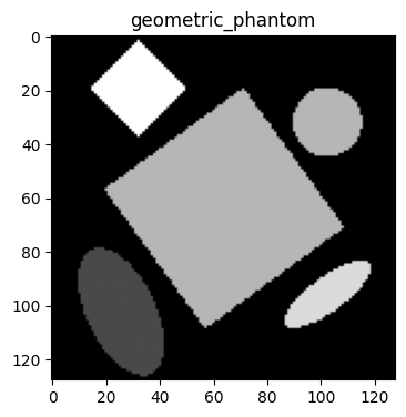
Example 4: Generate a geometric object phantom using the phantom simulation tool in BART#
Generate a geometric object phantom by using -G.#
geometric_phantom = bart(1, 'phantom -x 128 -G') # Generate a phantom image with size 128x128
# Visualizing the image using Matplotlib
plt.figure(figsize=(4,6))
plt.imshow(abs(geometric_phantom), cmap='gray')
plt.title('geometric_phantom')
Text(0.5, 1.0, 'geometric_phantom')
We can substitude -G by -T, --NIST, --SANAR, --BRAIN…
Option |
Description |
|---|---|
|
Geometric object phantom |
|
Tubes phantom |
|
NIST T2 sphere phantom |
|
Diagnostic SONAR phantom |
|
BRAIN geometry phantom |
|
Creates random tubes phantom with |
|
Generates the BART logo |
These commands can also be used with -s, -k, etc.
Example 5: Creating an Ellipsoid Phantom#
To create an ellipsoid, use --ELLIPSOID with additional options for setting its center and axes.
Command Explanation#
--ELLIPSOID: Specifies the ellipsoid geometry.--ellipsoid_center d:d:d: Sets the x, y, z coordinates of the ellipsoid’s center.--ellipsoid_axes f:f:f: Defines the lengths of the ellipsoid’s axes.
Run the following command to generate an ellipsoid phantom.
Example 5.1: Generate a Ellipsoid Phantom by using --ELLIPSOID.#
ellipsoid_phantom = bart(1, 'phantom -x 32 --ELLIPSOID') # Generate a ellipsoid image with size 32x32
# Visualizing the image using Matplotlib
plt.figure(figsize=(4,6))
plt.imshow(abs(ellipsoid_phantom), cmap='gray')
plt.title('ellipsoid')
Text(0.5, 1.0, 'ellipsoid')
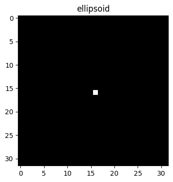
(You may notice this appears as a square rather than an ellipsoid; this is because the default ellipsoid axes are set to 1:1:1.)
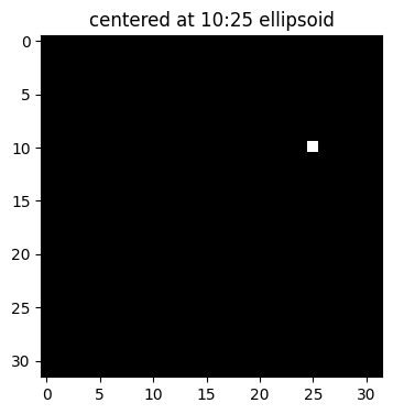
Example 5.1: Generate a Ellipsoid Phantom with Option for Setting Its Center#
--ELLIPSOID: Specifies the ellipsoid geometry.--ellipsoid_center d:d:d: Sets the x, y, z coordinates of the ellipsoid’s center.
ellipsoid_phantom_1 = bart(1, 'phantom -x 32 --ELLIPSOID --ellipsoid_center 10:25:1')
# Visualizing the image using Matplotlib
plt.figure(figsize=(4,6))
plt.imshow(abs(ellipsoid_phantom_1), cmap='gray')
plt.title('centered at 10:25 ellipsoid')
Text(0.5, 1.0, 'centered at 10:25 ellipsoid')
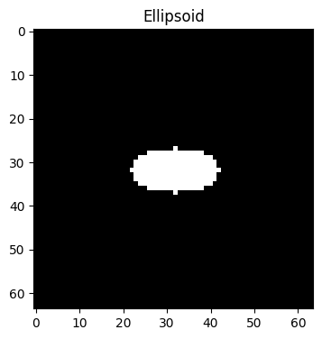
Example 5.2: Generate a Ellipsoid Phantom with Option for Setting Its lengths of the ellipsoid’s axes.#
--ELLIPSOID: Specifies the ellipsoid geometry.--ellipsoid_axes f:f:f: Defines the lengths of the ellipsoid’s axes.
ellipsoid_phantom_2 = bart(1, 'phantom -x 64 --ELLIPSOID --ellipsoid_axes 10:20:1') # The length for x is 10, for y is 20
# Visualizing the image using Matplotlib
plt.figure(figsize=(4,6))
plt.imshow(abs(ellipsoid_phantom_2), cmap='gray')
plt.title('Ellipsoid')
Text(0.5, 1.0, 'Ellipsoid')
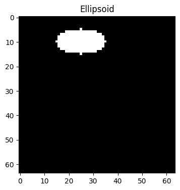
Example 5.3: Generate a Ellipsoid Phantom with Option for Setting Its Center and Axes.#
--ELLIPSOID: Specifies the ellipsoid geometry.--ellipsoid_center d:d:d: Sets the x, y, z coordinates of the ellipsoid’s center.--ellipsoid_axes f:f:f: Defines the lengths of the ellipsoid’s axes.
ellipsoid_phantom_3 = bart(1, 'phantom -x 64 --ELLIPSOID --ellipsoid_center 10:25:1, --ellipsoid_axes 10:20:1')
# Visualizing the image using Matplotlib
plt.figure(figsize=(4,6))
plt.imshow(abs(ellipsoid_phantom_3), cmap='gray')
plt.title('Ellipsoid')
Text(0.5, 1.0, 'Ellipsoid')
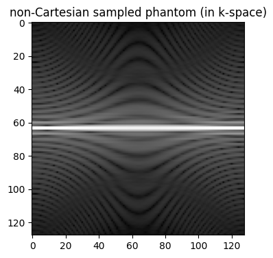
Example 6: Generate a k-space phantom by a trajectory file using the phantom simulation tool in BART#
Generates a radial k-space trajectory#
traj = bart(1, 'traj -r -x 128 -y 128')
Creates a simulated k-space dataset for a phantom image by the trajectory that we created#
traj_phantom_ksp = bart(1, 'phantom -k -t', traj)
# Visualizing the image using Matplotlib
plt.figure(figsize=(4,6))
plt.imshow(np.abs(traj_phantom_ksp.squeeze())**.3, cmap='gray')
plt.title('non-Cartesian sampled phantom (in k-space)')
Text(0.5, 1.0, 'non-Cartesian sampled phantom (in k-space)')
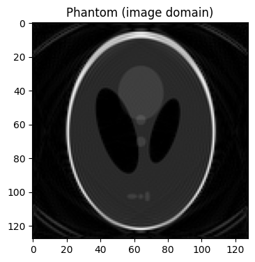
# Visualizing the inverse NUFFT using Matplotlib
traj_phantom_img = bart(1, 'nufft -i', traj, traj_phantom_ksp)
plt.figure(figsize=(4,6))
plt.imshow(np.abs(traj_phantom_img), cmap='gray')
plt.title('Phantom (image domain)')
Est. image size: 128x128x1
Done.
Text(0.5, 1.0, 'Phantom (image domain)')
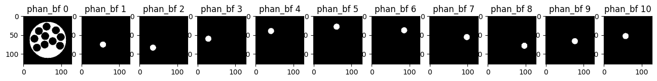
Example 7: Generate Tube phantom image by basis functions of geometry using the phantom simulation tool in BART#
# Generates a 128 × 128 phantom image of cylindrical tubes using basis functions for geometry representation
phantom_bf = bart(1, 'phantom -x 128 -b -T').squeeze()
# Visualizing the the images using Matplotlib
plt.figure(figsize=(16,25))
for i in range(11):
    plt.subplot(1, 11, i+1)
    plt.imshow(abs(phantom_bf[...,i]), cmap='gray')
    plt.title('phan_bf {}'.format(i))
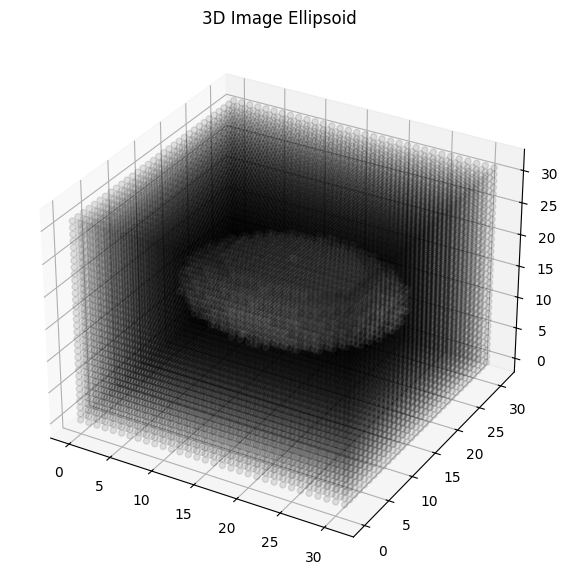
Example 8: Generate a 3D phantom using the phantom simulation tool in BART#
Generate a 3D phantom with an ellipsoid geometry by option#
-3: 3D--ELLIPSOID: Specifies the ellipsoid geometry.--ellipsoid_axes f:f:f: Defines the lengths of the ellipsoid’s axes.
# Generate a 3D phantom of size 32 × 32 × 32 with an ellipsoid geometry, specifying the ellipsoid's axes lengths as 10 × 20 × 10
phantom_3d = bart(1, 'phantom -x 32 -3 --ELLIPSOID --ellipsoid_axes 20:25:10')
# Visualizing the the images using Matplotlib
from mpl_toolkits.mplot3d import Axes3D  # Import the 3D plotting functionality from the matplotlib library.

# Define a grid of x, y, z coordinates
x, y, z = np.meshgrid(np.arange(phantom_3d.shape[0]),
                      np.arange(phantom_3d.shape[1]),
                      np.arange(phantom_3d.shape[2]))

# Use the magnitude of the complex data
magnitude = np.abs(phantom_3d)

# Plot the 3D image as scatter points
fig = plt.figure(figsize=(7, 7))
ax = fig.add_subplot(111, projection='3d')
scat = ax.scatter(x, y, z, c=magnitude.flatten(), cmap='gray', marker='o', alpha=0.1)

ax.set_title("3D Image Ellipsoid")
plt.show()
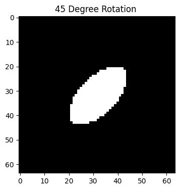
Example 9: Generate a rotation phantom using the phantom simulation tool in BART#
Generate a rotated ellipsoid phantom by option#
--ELLIPSOID: Specifies the ellipsoid geometry.--ellipsoid_axes f:f:f: Defines the lengths of the ellipsoid’s axes.-rotation-angle [deg]: [deg] defines angle of rotation
# Generates a ellipsoid phantom of size 64 × 64 × 64 with axes 30 x 15, and rotated by 45 degrees.
phantom_rotation = bart(1, 'phantom -x 64 --ELLIPSOID --ellipsoid_axes 30:15:1 --rotation-angle 45')
# Visualizing the image using Matplotlib
plt.figure(figsize=(4,6))
plt.imshow(abs(phantom_rotation), cmap='gray')
plt.title('45 Degree Rotation ')
Text(0.5, 1.0, '45 Degree Rotation ')
Example 10: Generate a 2D head coil configuration supporting up to 8 channels phantom using the phantom simulation tool in BART#
phantom_coil = bart(1, 'phantom --coil HEAD_2D_8CH')
# Visualizing the image using Matplotlib
plt.figure(figsize=(4,6))
plt.imshow(abs(phantom_coil), cmap='gray')
plt.title('Coil HEAD_2D_8CH')
Text(0.5, 1.0, 'Coil HEAD_2D_8CH')

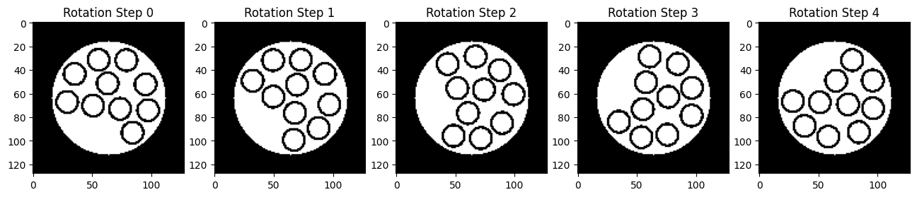
Example 11: Generate a rotation tube phantom using the phantom simulation tool in BART#
Generate a rotated tube phantom with rotation steps by option#
-rotation-angle [deg]: [deg] defines angle of rotation--rotation-steps: n – Number of rotation steps-T: Tubes phantom
phantom_rs = bart(1, 'phantom -x 128 -T --rotation-angle 30 --rotation-steps 5').squeeze()
# Visualizing the multi-coil images using Matplotlib
plt.figure(figsize=(16,20))
for i in range(5):
    plt.subplot(1, 5, i+1)
    plt.imshow(abs(phantom_rs[...,i]), cmap='gray')
    plt.title('Rotation Step {}'.format(i))