bart avg#
===========================================================================================================
The bart avg command is used to average along a specific dimension of multi-dimensional arrays using a bitmask.
Where we can view the full usage string and optional arguments with the -h flag.
How bart avg Works#
The averaging process computes the mean value along the specified dimension(s). If you want to average over a given dimension, the formula is:
where:
\(N\) is the number of elements along the dimension to be averaged.
\(x_i\) represents the individual data points in the dimension being averaged.
!bart avg -h
Usage: avg [-w] bitmask <input> <output>

Calculates (weighted) average along dimensions specified by bitmask.

-w    weighted average
-h    help
Where:
-w: This option enables weighted averaging.
bitmask: A bitmask to specify the dimensions along which to perform the averaging.
<input>: The input .cfl file.
<output>: The output .cfl file containing the averaged data.
Example for Matrix (using Bash)#
Create a Matrix, Dimension as 2 x 2 x 2#
!bart vec $(seq 1 8) array # Generate a array with values from 1 to 8
!bart show array
+1.000000e+00+0.000000e+00i	+2.000000e+00+0.000000e+00i
+3.000000e+00+0.000000e+00i	+4.000000e+00+0.000000e+00i
+5.000000e+00+0.000000e+00i	+6.000000e+00+0.000000e+00i
+7.000000e+00+0.000000e+00i	+8.000000e+00+0.000000e+00i
!bart reshape $(bart bitmask 0 1 2) 2 2 2 array matrix_array # Reshape the array to Dimension as 2 x 2 x 2
!bart show matrix_array
+1.000000e+00+0.000000e+00i +2.000000e+00+0.000000e+00i
+3.000000e+00+0.000000e+00i +4.000000e+00+0.000000e+00i
+5.000000e+00+0.000000e+00i +6.000000e+00+0.000000e+00i
+7.000000e+00+0.000000e+00i +8.000000e+00+0.000000e+00i
!bart show -m matrix_array
Type: complex float
Dimensions: 16
AoD:	2	2	2	1	1	1	1	1	1	1	1	1	1	1	1	1
Example 1.1#
Calculated the Average Along a Dimension “0” of the matrix_array#
!bart avg $(bart bitmask 0) matrix_array matrix1_array
!bart show matrix1_array
+1.500000e+00+0.000000e+00i	+3.500000e+00+0.000000e+00i
+5.500000e+00+0.000000e+00i	+7.500000e+00+0.000000e+00i
We can see the dimension for our new matrix (matrix1_array) become 1 x 2 x 2
!bart show -m matrix1_array
Type: complex float
Dimensions: 16
AoD:	1	2	2	1	1	1	1	1	1	1	1	1	1	1	1	1
Example 1.2#
Continue to Calculate avg for matrix1_arry along Demension “2”#
!bart avg $(bart bitmask 2) matrix1_array matrix2_array
!bart show matrix2_array
+3.500000e+00+0.000000e+00i +5.500000e+00+0.000000e+00i
!bart show -m matrix2_array
Type: complex float
Dimensions: 16
AoD:	1	2	1	1	1	1	1	1	1	1	1	1	1	1	1	1
Example 1.3#
Calculate the avg Across all Dimensions of a Matrix using BART#
!bart avg $(bart bitmask 0 1 2) matrix_array matrix3_array
!bart show matrix3_array
+4.500000e+00+0.000000e+00i
!bart show -m matrix3_array
Type: complex float
Dimensions: 16
AoD:	1	1	1	1	1	1	1	1	1	1	1	1	1	1	1	1
Example Workflow for Images (in Python Kernel)#
The bart avg command in BART is often used to calculate the Average data across one or more specified dimensions. It is typically employed in cases where multi-dimensional data, such as MRI data, needs to be averaged along specific axes, such as repetitions, coils, or slices.
Example in Coils#
# Importing the required libraries
import numpy as np
import matplotlib.pyplot as plt
%matplotlib inline

import cfl
from bart import bart
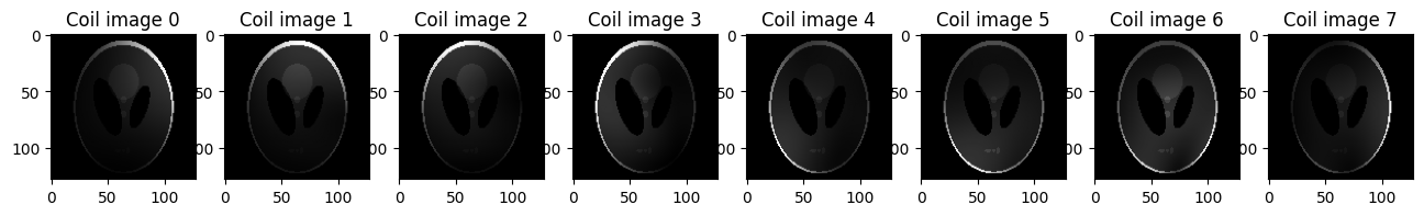
1. Generate a multi-coil image using the phantom simulation tool in BART:#
Generate a multi-coil image with size 128x128 and 8 coils.
Note the convention is that the coil dimension is dimension 3
# Generate a multi-coil image with size 128x128 and 8 coils
multi_coil_image = bart(1, 'phantom -x 128 -s 8')
print(multi_coil_image.shape)
(128, 128, 1, 8)
# Visualizing the multi-coil images using Matplotlib
plt.figure(figsize=(16,20))
for i in range(8):
    plt.subplot(1, 8, i+1)
    plt.imshow(abs(multi_coil_image[...,i]), cmap='gray')
    plt.title('Coil image {}'.format(i))
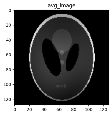
2. Combine the Coil Images Using avg :#
The number of coils is located in dimension 3, and the corresponding bitmask for dimension 3 is calculated to be 8
!bart bitmask 3
8
avg_image = bart(1, 'avg 8', multi_coil_image) # Calculates the avg across coil dimension and named as avg_image
# Visualizing the avg_image using Matplotlib
plt.figure(figsize=(4,6))
plt.imshow(abs(avg_image), cmap='gray')
plt.title('avg_image')
Text(0.5, 1.0, 'avg_image')